5.7 Drawing Free-Body Diagrams

Learning Objectives

By the end of this section, you will be able to:

Explain the rules for drawing a free-body diagram
Construct free-body diagrams for different situations

The first step in describing and analyzing most phenomena in physics involves the careful drawing of a free-body diagram. Free-body diagrams have been used in examples throughout this chapter. Remember that a free-body diagram must only include the external forces acting on the body of interest. Once we have drawn an accurate free-body diagram, we can apply Newton’s first law if the body is in equilibrium (balanced forces; that is, $F_{net} = 0$ ) or Newton’s second law if the body is accelerating (unbalanced force; that is, $F_{net} \neq 0$ ).

In Forces, we gave a brief problem-solving strategy to help you understand free-body diagrams. Here, we add some details to the strategy that will help you in constructing these diagrams.

Problem-Solving Strategy

Constructing Free-Body Diagrams

Observe the following rules when constructing a free-body diagram:

Draw the object under consideration; it does not have to be artistic. At first, you may want to draw a circle around the object of interest to be sure you focus on labeling the forces acting on the object. If you are treating the object as a particle (no size or shape and no rotation), represent the object as a point. We often place this point at the origin of an xy-coordinate system.
Include all forces that act on the object, representing these forces as vectors. Consider the types of forces described in Common Forces—normal force, friction, tension, and spring force—as well as weight and applied force. Do not include the net force on the object. With the exception of gravity, all of the forces we have discussed require direct contact with the object. However, forces that the object exerts on its environment must not be included. We never include both forces of an action-reaction pair.
Convert the free-body diagram into a more detailed diagram showing the x- and y-components of a given force (this is often helpful when solving a problem using Newton’s first or second law). In this case, place a squiggly line through the original vector to show that it is no longer in play—it has been replaced by its x- and y-components.
If there are two or more objects, or bodies, in the problem, draw a separate free-body diagram for each object.

Note: If there is acceleration, we do not directly include it in the free-body diagram; however, it may help to indicate acceleration outside the free-body diagram. You can label it in a different color to indicate that it is separate from the free-body diagram.

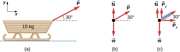
Let’s apply the problem-solving strategy in drawing a free-body diagram for a sled. In Figure 5.31(a), a sled is pulled by force P at an angle of $30 °$ . In part (b), we show a free-body diagram for this situation, as described by steps 1 and 2 of the problem-solving strategy. In part (c), we show all forces in terms of their x- and y-components, in keeping with step 3.

Figure a shows a sled of 15 kg. An arrow labeled P pointing right and up forms an angle of 30 degrees with the horizontal. Figure b is a free body diagram with P, N pointing up and w pointing down. Figure c is a free body diagram with P, N, w and two components of P: Px pointing right and Py pointing up.

Figure 5.31 (a) A moving sled is shown as (b) a free-body diagram and (c) a free-body diagram with force components.

Example 5.14

Two Blocks on an Inclined Plane

Construct the free-body diagram for object A and object B in Figure 5.32.

Strategy

We follow the four steps listed in the problem-solving strategy.

Solution

We start by creating a diagram for the first object of interest. In Figure 5.32(a), object A is isolated (circled) and represented by a dot.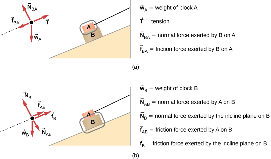

Figure a shows two objects on an inclined plane, sloping down to the left. Object A is on top of object B. A free body diagram shows T pointing right and up, parallel to the plane, N subscript BA pointing left and up, perpendicular to the plane, f subscript BA pointing left and down, parallel to the plane and w subscript A pointing vertically down. W subscript A is weight of block A, T is tension, N subscript BA is normal force exerted by B on A, f subscript BA is friction force exerted by B on A. Figure b shows the objects on the slope in the same manner. A free body diagram has f subscript B and f subscript AB pointing right and up, parallel to the slope, N subscript B pointing left and up perpendicular to the slope, w subscript B pointing vertically down and N subscript AB pointing down and right, perpendicular to the slope. W subscript B is weight of block B, N subscript AB is normal force exerted by A on B, N subscript B is normal force exerted by the incline plane on B. f subscript AB is friction force exerted by A on B. f subscript B is friction force exerted by the incline plane on B.

Figure 5.32 (a) The free-body diagram for isolated object A. (b) The free-body diagram for isolated object B. Comparing the two drawings, we see that friction acts in the opposite direction in the two figures. Because object A experiences a force that tends to pull it to the right, friction must act to the left. Because object B experiences a component of its weight that pulls it to the left, down the incline, the friction force must oppose it and act up the ramp. Friction always acts opposite the intended direction of motion.

We now include any force that acts on the body. Here, no applied force is present. The weight of the object acts as a force pointing vertically downward, and the presence of the cord indicates a force of tension pointing away from the object. Object A has one interface and hence experiences a normal force, directed away from the interface. The source of this force is object B, and this normal force is labeled accordingly. Since object B has a tendency to slide down, object A has a tendency to slide up with respect to the interface, so the friction $f_{BA}$ is directed downward parallel to the inclined plane.

As noted in step 4 of the problem-solving strategy, we then construct the free-body diagram in Figure 5.32(b) using the same approach. Object B experiences two normal forces and two friction forces due to the presence of two contact surfaces. The interface with the inclined plane exerts external forces of $N_{B}$ and $f_{B}$ , and the interface with object B exerts the normal force $N_{AB}$ and friction $f_{AB}$ ; $N_{AB}$ is directed away from object B, and $f_{AB}$ is opposing the tendency of the relative motion of object B with respect to object A.

Significance

The object under consideration in each part of this problem was circled in gray. When you are first learning how to draw free-body diagrams, you will find it helpful to circle the object before deciding what forces are acting on that particular object. This focuses your attention, preventing you from considering forces that are not acting on the body.

Example 5.15

Two Blocks in Contact

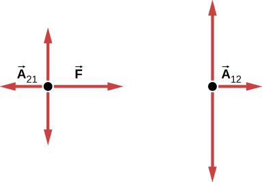
A force is applied to two blocks in contact, as shown. Draw the reaction forces between the two blocks.

Strategy

Draw a free-body diagram for each block. Be sure to consider Newton’s third law at the interface where the two blocks touch.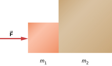 Two squares are shown in contact with each other. The left one is smaller and is labeled m1. The right one is bigger and is labeled m2. An arrow pointing right towards m1 is labeled F.

Two squares are shown in contact with each other. The left one is smaller and is labeled m1. The right one is bigger and is labeled m2. An arrow pointing right towards m1 is labeled F.

Solution

Figure shows two free body diagrams. The first one shows arrow A subscript 21 pointing left and arrow F pointing right. The second one shows arrow A 12 pointing right. Both diagrams also have arrows pointing up and down.

Significance

{\vec{A}}_{21}

is the action force of block 2 on block 1.

{\vec{A}}_{12}

is the reaction force of block 1 on block 2. We use these free-body diagrams in Applications of Newton’s Laws.

Example 5.16

Block on the Table (Coupled Blocks)

A block rests on the table, as shown. A light rope is attached to it and runs over a pulley. The other end of the rope is attached to a second block. The two blocks are said to be coupled. Block

m_{2}

exerts a force due to its weight, which causes the system (two blocks and a string) to accelerate.

Strategy

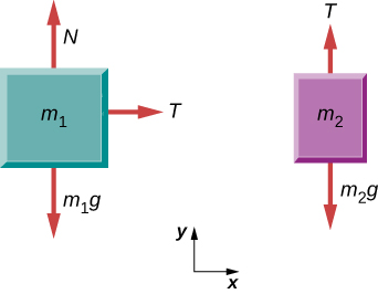
We assume that the string has no mass so that we do not have to consider it as a separate object. Draw a free-body diagram for each block.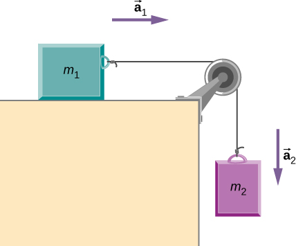 Figure shows block m1 placed on a table. A string attached to it runs over a pulley and down the right side of the table. A block m2 is suspended from it. An arrow a1 points right and an arrow a2 points down.

Figure shows block m1 placed on a table. A string attached to it runs over a pulley and down the right side of the table. A block m2 is suspended from it. An arrow a1 points right and an arrow a2 points down.

Solution

Figure a shows block m1. An arrow labeled N point upwards from it, an arrow m1g points downwards and an arrow T points right. Figure b shows block m2. An arrow T points upwards from it and an arrow m2g points downwards.

Significance

Each block accelerates (notice the labels shown for

{\vec{a}}_{1}

and

{\vec{a}}_{2}

); however, assuming the string remains taut, the magnitudes of acceleration are equal. Thus, we have

| {\vec{a}}_{1} | = | {\vec{a}}_{2} |

. If we were to continue solving the problem, we could simply call the acceleration

\vec{a}

. Also, we use two free-body diagrams because we are usually finding tension T, which may require us to use a system of two equations in this type of problem. The tension is the same on both

m_{1} and m_{2}

Check Your Understanding 5.10

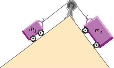
(a) Draw the free-body diagram for the situation shown. (b) Redraw it showing components; use x-axes parallel to the two ramps.

Two carts are tied with a rope which goes over a pulley on top of a hill. Each cart rests on one slope of the hill on either side of the pulley. The cart on the left is labeled m1 and the one on the right is labeled m2.

Numerical Methods Example

Now that we have explored different kinds of forces, let's see an example of how we could use computational methods to simulate a more realistic problem. Suppose we have an object that is experiencing a spring-like restoring force, and a friction force. For simplicity we will assume the equilibrium position of the spring-like force is at $x = 0$ . To make it a little more realistic, we will use a friction force that depends on velocity. Not all friction forces we deal with work this way, but for the sake of this problem, this is the kind we will use at the moment.

Let the spring-like force be given by $F_{spring} = - k x$ where $k =$ 1 N/m. Notice that the direction of the force is opposite the direction of the displacement (as determined by the minus sign). Let the friction force be given by $f = - b v$ where $b =$ 0.01 newton-seconds per meter. This friction force is opposite to the direction of motion (as described by the minus sign).

Suppose the object (with mass $m =$ 10 grams) starts with an initial velocity of zero and an initial displacement of $x_{0} =$ 20 centimeters. We wish to graph the position vs time function and be able to describe the motion. For this we will use our knowledge of forces to determine the acceleration. We will then use Euler's method to determine the position vs time function from the acceleration.

Using Newton's second law, we know that $\sum F = m a$ . Since we only have two forces, plugging both of them in gives us $- k x - b v = m a$ . To solve for acceleration, all we need to do is divide by the mass of the object. Now that we have acceleration, we can put it into our Euler's method code. However, notice that this acceleration depends on position and velocity rather than time, so we will need to make those the inputs of our acceleration function.

# define knowns k = 1 # N/m b = 0.01 # Ns/m m = 0.01 # kg x0 = 0.2 # m # define acceleration (function of position and velocity) def a(x, v): return -(k*x + b*v)/m # set up Euler's method x = x0 # initial position v = 0 # initial velocity t = 0 # start timer at 0 dt = 0.001 # time step # lists for plotting xpoints = [] tpoints = [] while t < 10: # run for 10 seconds # save current state to list xpoints.append(x) tpoints.append(t) # update position with velocity x += v*dt # += means add that much # update velocity with acceleration v += a(x, v)*dt # a takes in current x and current v # update timer t += dt # now plot the results from matplotlib import pyplot as plt plt.clf() plt.plot(tpoints, xpoints) plt.title('Position vs Time of Dampened Harmonic Oscillator') plt.xlabel('Time (s)') plt.ylabel('Position (m)') plt.show()

This system is called a dampened harmonic oscillator, and it shows up in all sorts of places in the real world. The spring-like force creates an oscillation motion, while the friction force creates dampening. You will likely explore this system more in your future. It is an important application of Newton's second law and of forces because it is so applicable. In many real world systems, we may either want to avoid/dampen as much as we can the oscillations that naturally occur, or allow them to happen. Understanding where it comes from is a crutial first step.

Interactive

Engage the simulation below to predict, qualitatively, how an external force will affect the speed and direction of an object’s motion. Explain the effects with the help of a free-body diagram. Use free-body diagrams to draw position, velocity, acceleration, and force graphs, and vice versa. Explain how the graphs relate to one another. Given a scenario or a graph, sketch all four graphs.