3.6 Finding Velocity and Displacement from Acceleration

Learning Objectives

By the end of this section, you will be able to:

Derive the kinematic equations for constant acceleration using integral calculus.
Use the integral formulation of the kinematic equations in analyzing motion.
Find the functional form of velocity versus time given the acceleration function.
Find the functional form of position versus time given the velocity function.

This section assumes you have enough background in calculus to be familiar with integration. In Instantaneous Velocity and Speed and Average and Instantaneous Acceleration we introduced the kinematic functions of velocity and acceleration using the derivative. By taking the derivative of the position function we found the velocity function, and likewise by taking the derivative of the velocity function we found the acceleration function. Using integral calculus, we can work backward and calculate the velocity function from the acceleration function, and the position function from the velocity function.

Kinematic Equations from Integral Calculus

Let’s begin with a particle with an acceleration a(t) which is a known function of time. Since the time derivative of the velocity function is acceleration,

\frac{d}{d t} v (t) = a (t),

we can take the indefinite integral of both sides, finding

\int \frac{d}{d t} v (t) d t = \int a (t) d t + C_{1},

where C₁ is a constant of integration. Since $\int \frac{d}{d t} v (t) d t = v (t)$ , the velocity is given by

v (t) = \int a (t) d t + C_{1} .

3.18

Similarly, the time derivative of the position function is the velocity function,

\frac{d}{d t} x (t) = v (t) .

Thus, we can use the same mathematical manipulations we just used and find

x (t) = \int v (t) d t + C_{2},

3.19

where C₂ is a second constant of integration.

We can derive the kinematic equations for a constant acceleration using these integrals. With a(t) = a a constant, and doing the integration in Equation 3.18, we find

v (t) = \int a d t + C_{1} = a t + C_{1} .

If the initial velocity is v(0) = v₀, then

v_{0} = 0 + C_{1} .

Then, C₁ = v₀ and

v (t) = v_{0} + a t,

which is Equation 3.12. Substituting this expression into Equation 3.19 gives

x (t) = \int (v_{0} + a t) d t + C_{2} .

Doing the integration, we find

x (t) = v_{0} t + \frac{1}{2} a t^{2} + C_{2} .

If x(0) = x₀, we have

x_{0} = 0 + 0 + C_{2};

so, C₂ = x₀. Substituting back into the equation for x(t), we finally have

x (t) = x_{0} + v_{0} t + \frac{1}{2} a t^{2},

which is Equation 3.13.

Example 3.17

Motion of a Motorboat

A motorboat is traveling at a constant velocity of 5.0 m/s when it starts to accelerate opposite to the motion to arrive at the dock. Its acceleration is

a (t) = - \frac{1}{4} t m/ s^{3}

. (a) What is the velocity function of the motorboat? (b) At what time does the velocity reach zero? (c) What is the position function of the motorboat? (d) What is the displacement of the motorboat from the time it begins to accelerate opposite to the motion to when the velocity is zero? (e) Graph the velocity and position functions.

Strategy

(a) To get the velocity function we must integrate and use initial conditions to find the constant of integration. (b) We set the velocity function equal to zero and solve for t. (c) Similarly, we must integrate to find the position function and use initial conditions to find the constant of integration. (d) Since the initial position is taken to be zero, we only have to evaluate the position function at the time when the velocity is zero.

Solution

We take t = 0 to be the time when the boat starts to accelerate opposite to the motion.

From the functional form of the acceleration we can solve Equation 3.18 to get v(t):
$v (t) = \int a (t) d t + C_{1} = \int - \frac{1}{4} t m/ s^{3} d t + C_{1} = - \frac{1}{8} m/ s^{3} t^{2} + C_{1} .$
At t = 0 we have v(0) = 5.0 m/s = 0 + C₁, so C₁ = 5.0 m/s or $v (t) = 5.0 m/ s - \frac{1}{8} m/ s^{3} t^{2}$ .
$v (t) = 0 = 5.0 m/ s - \frac{1}{8} t^{2} m/ s^{3} \Rightarrow t = 6.3 s$
Solve Equation 3.19:
$x (t) = \int v (t) d t + C_{2} = \int (5.0 - \frac{1}{8} t^{2}) d t + C_{2} = 5.0 t m/s - \frac{1}{24} t^{3} m/ s^{3} + C_{2} .$
At t = 0, we set x(0) = 0 = x₀, since we are only interested in the displacement from when the boat starts to accelerate opposite to the motion. We have
$x (0) = 0 = C_{2} .$
Therefore, the equation for the position is
$x (t) = 5.0 t m/s - \frac{1}{24} t^{3} m/ s^{3} .$
Since the initial position is taken to be zero, we only have to evaluate the position function at the time when the velocity is zero. This occurs at t = 6.3 s. Therefore, the displacement is
$x (6.3) = 5.0 t m/s (6.3 s) - \frac{1}{24} t^{3} m/ s^{s} (6.3 s)^{3} = 21.1 m .$

Graph A is a plot of velocity in meters per second as a function of time in seconds. Velocity is five meters per second at the beginning and decreases to zero. Graph B is a plot of position in meters as a function of time in seconds. Position is zero at the beginning, increases reaching maximum between six and seven seconds, and then starts to decrease.

Figure 3.30 (a) Velocity of the motorboat as a function of time. The motorboat decreases its velocity to zero in 6.3 s. At times greater than this, velocity becomes negative—meaning, the boat is reversing direction. (b) Position of the motorboat as a function of time. At t = 6.3 s, the velocity is zero and the boat has stopped. At times greater than this, the velocity becomes negative—meaning, if the boat continues to move with the same acceleration, it reverses direction and heads back toward where it originated.

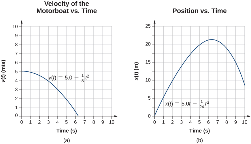
Significance

The acceleration function is linear in time so the integration involves simple polynomials. In Figure 3.30, we see that if we extend the solution beyond the point when the velocity is zero, the velocity becomes negative and the boat reverses direction. This tells us that solutions can give us information outside our immediate interest and we should be careful when interpreting them.

Check Your Understanding 3.8

A particle starts from rest and has an acceleration function $a (t) = (5 - (10 \frac{1}{s}) t) \frac{m}{s^{2}}$ . (a) What is the velocity function? (b) What is the position function? (c) When is the velocity zero?

Integration In Python

In previous section of this chapter we introduced functions as a tool to allow us to compute the derivative of a function in Python. This allowed us to determine the velocity vs time and the acceleration vs time graphs from just the position function. There are several methods for using code to go the other way, starting with acceleration and determining position. One simple yet powerful one that we will explore briefly in this course is called Euler's method (pronounced "Oi-lers"). Euler's method won't give us the equation for position, but it can be useful when we need to make a graph or calculate a number.

Euler's method is about breaking a big problem into many smaller connected problems. Up to now, most of our code has not been too lengthly. Euler's method can come with a bit of a learning curve though because as we solve these many small connected problems, we have to keep track of the answers in a way such that we can reuse them later. In order to give it proper attention to all the pieces, Euler's method is explained in detail in the next section.

Numerical Method Example

Let us consider the motorboat from Example 3.17. Its acceleration is $a (t) = - \frac{1}{4} t m/ s^{3}$ . It has an initial velocity of 5 m/s and we will take its initial position to be 0. We wish to find the velocity and position functions, and the time when the velocity is zero. For this we will use Euler's method. The code below uses Euler's method to make a plot of the velocity and position functions.

# define knowns def a(t): return -0.25*t # defining acceleration as a function v = 5 # start v as 5 m/s x = 0 # start x as 0 m t = 0 # start timer at 0 # make some lists for plotting tpoints = [] # start them empty xpoints = [] vpoints = [] # time step dt = 0.001 # now loop through while t < 10: # loop for 10 seconds # add stuff to the plotting lists tpoints.append(t) xpoints.append(x) vpoints.append(v) # update position using velocity x = x + v*dt # update velocity using acceleration v = v + a(t)*dt # plug current t into the acceleration function # update timer t = t + dt # now the simulation is done. Plot the results from matplotlib import pyplot as plt fig, ax = plt.subplots(nrows=1, ncols=2, figsize=(10, 4)) ax[0].plot(tpoints, vpoints) ax[0].set_title('Velocity vs Time') ax[0].set_xlabel('Time (s)') ax[0].set_ylabel('Velocity (m/s)') ax[1].plot(tpoints, xpoints) ax[1].set_title('Position vs Time') ax[1].set_xlabel('Time (s)') ax[1].set_ylabel('Position (m)') plt.show() # print the max of position to give us the location from numpy import argmax print(f'The velocity is zero at {tpoints[xpoints.index(max(xpoints))]:.2g} s.') print(f'The location at that that time is {max(xpoints):.3g} m.')

We see that by simulating the acceleration, we were able to arrive at the same answer as given in the example earlier. While this may not be the easier method for simple problems, in general acceleration may not be able to be integrated by hand, while integrating numerically like this will always give us an answer.